In AI, sometimes, you need to plan a sequence of action that lead you to your goal. In stochastic environment, in those situation where you can’t know the outcomes of your actions, a sequence of actions is not sufficient: you need a policy.
Markov Decision Process
is a mathematical framework that helps to build a policy in a stochastic environment where you know the probabilities of certain outcomes.
In this post, I give you a breif introduction of Markov Decision Process. Then, I’ll show you my implementation, in python, of the most important algorithms that can help you to find policies in stocastic enviroments. You can fine a more detailed description of the Markov Decision Process in my
my slides
that I’ve used for a seminar at University.
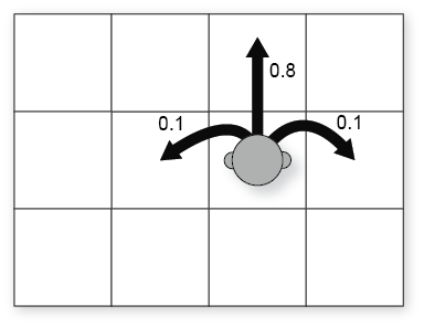
To explain the Markov Decision Process, we use the same environment example of the book “Artificial Intelligence: A Modern Approach (3rd ed.)”. This environment is called Grid World, it is a simple grid environment where the possible actions are NORTH, SOUTH, EAST, WEST. Assume that the probability to go forward is 0.8 and the probability to go left or right is 0.1.
For example, if you are in the cell (2,1) and you want to do the action “NORTH” the possible outcomes can be represented as the following:
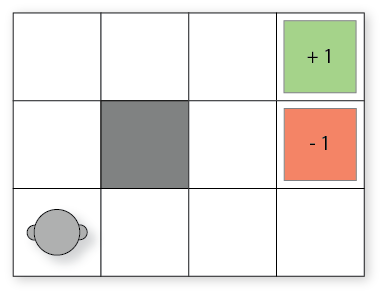
We need a goal: the grid world have an exit with an utility of +1. But, there are some pits that have an utility of -1. Each the exit and the pit are terminal cells (i.e. we cannot do any action from them). We can’t go out of the grid and we can use walls to have more spatial constraints.
To build the policy, we need an estimation of the utilities of each cell. We can calculate these utilities using a method like
minimax
: this method is called
expectiminimax
. But some applications (i.e. if you don’t have terminal states), sometimes this method is infeasible.
Markov decision process helps us to calculate these utilities, with some powerful methods.
To understand the concepts on the books, I’ve written a simple script in python to “touch” the theory. I’ll show you the basic concepts to understand the code.
Policy Iteration and Value Iteration
First of all, we have a class called GridWorld, with this class we model our
grid world.
def transitionFunction(self, position, action):
    ''' this function describes the movements that we can do (deterministic)
        if we are in a pit, in a exit or in a wall cell we can't do anything
        we can't move into a wall
        we can't move out the border of the grid
        returns the new position
    '''
def possiblePositionsFromAction(self, position, worldAction):
    ''' given an action worldAction, return a dictionary D,
        where for each action a, D[a] is the probability to do the action a
    '''
With these methods we model the deterministic actions (transitionFunction) and
the stochastic actions (possiblePositionsFromAction). The other methods of the
class are simple to understand.
We must build a policy, to do this we have another class called Policy that
implements the two ways to build the policy: Value Iteration and Policy
Iteration.
Value Iteration
The following method implements the Value Iteration algorithm. I show you a simplified version of the algorithm, that hides some difficult peculiarities.
def valueIteration(self):
    '''using the Value Iteration algorithm (see AI: A Modern Approach (3rd ed.) pag. 652)
        calculate the utilities for all states in the grid world

        the algorithm has a maximum number of iterations, in this way we can compute an
        example with a discount factor = 1 that converge.

        returns the number of iterations it needs for converge
    '''

    eps = Policy.valueIterationEepsilon
    dfact = self.world.discFactor
    c, r = self.world.size

    reiterate = True
    while(reiterate):
        self.numOfIterations += 1
        maxNorm = 0 #see the max norm definition in AI: A Modern Approach (3rd ed.) pag. 654

        newUv = self.__createEmptyUtilityVector()

        for x in range(c):
            for y in range(r):
                v = self.__cellUtility(x, y) #calculate using the self.utilities (i.e. the previous step)
                if not v is None: maxNorm = max(maxNorm, abs(self.utilities[y][x] - v))
                    newUv[y][x] = v #update the new utility vector that we are creating

                self.utilities = newUv

                if maxNorm <= eps * (1 - dfact)/dfact: reiterate = False
                if self.numOfIterations >= Policy.maxNumberOfIterations:
                    reiterate = False

    return self.numOfIterations
What we do is to iterate the Bellman Update (i.e. self.__cellUtility(x, y))
until we converge. We can see that the code is very simple to understand, the
concept of iterate a function until we converge is itself a simple thing. The
Bellman Update can be implemented as the following:
def __cellUtility(self, x, y):
    '''calculate the utility of a function using an utilities that is less precise (i.e. using the
       utility vector of the previous step.
    '''
    if self.world.cellAt(x,y) == GridWorld.CELL_VOID:
        maxSum = None
        for action in GridWorld.actionSet:
            summ = 0
            possibilities = self.world.possiblePositionsFromAction((x,y), action)
            for _, nextPos, prob in possibilities:
                summ += prob * self.utilities[nextPos[1]][nextPos[0]]
            if (maxSum is None) or (summ > maxSum): maxSum = summ
        res = self.world.rewardAtCell(x, y) + self.world.discFactor * maxSum
    else:
        #we don't have any action to do, we have only own reward (i.w. V*(s) = R(s) + 0)
        res = self.world.rewardAtCell(x, y)
    return res
Note that we use the methods of the grid world to know the possible outcomes of an action. The Bellman update can be seen in “AI: A Modern Approach (3rd ed.)” pag. 652.
Policy Iteration
The policy iteration is harder to understand. First of all, we need a random policy for the first step, using the following method:
def __createEmptyPolicy(self):
    '''we create a partial function that is undefined in all points'''
    c, r = self.world.size
    return [ [ (None if self.world.cellAt(x,y) == GridWorld.CELL_VOID else GridWorld.randomAction()) for x in range(c) ] for y in range(r) ]
Then we can write the policy iteration. It iterate the Policy Evaluation that update the utility vector given fixed policy. We iterate it until we reach a fixed point of the policy (i.e. the policy at step i is the same of the policy at step i+1).
def policyIteration(self):
    '''returns the number of iterations it needs to find the fixed point'''

    c, r = self.world.size
    policy = self.__createEmptyPolicy()

    reiterate = True
    while(reiterate):
        self.numOfIterations += 1

        self.policyEvaluation(policy)

        someChanges = False
        for x in range(c):
            for y in range(r):
                if self.world.cellAt(x,y) == GridWorld.CELL_VOID:
                    newMax = None
                    argMax = None
                    for action in GridWorld.actionSet:
                        summ = 0
                        possibilities = self.world.possiblePositionsFromAction((x,y), action)
                        for _, nextPos, prob in possibilities:
                            summ += prob * self.utilities[nextPos[1]][nextPos[0]]
                        if (newMax is None) or (summ > newMax):
                            argMax = action
                            newMax = summ

                    summ = 0
                    possibilities = self.world.possiblePositionsFromAction((x,y), policy[y][x])
                    for _, nextPos, prob in possibilities:
                        summ += prob * self.utilities[nextPos[1]][nextPos[0]]
                    if newMax > summ:
                        policy[y][x] = argMax
                        someChanges = True

        reiterate = someChanges
        if self.numOfIterations >= Policy.maxNumberOfIterations:
            reiterate = False

    return self.numOfIterations
The pseudo-code of this implementation can be found at “AI: A Modern Approach (3rd ed.)” at pag. 656. The algorithm use the Policy Evaluation: it is similar to the Value Iteration, but simpler because it use a fixed policy.
def policyEvaluation(self, policy):
    '''Policy Evaluation (see AI: A Modern Approach (3rd ed.) pag. 656)'''

    eps = Policy.valueIterationEepsilon
    dfact = self.world.discFactor
    c, r = self.world.size

    numOfIterations = 0
    reiterate = True
    while(reiterate):
        maxNorm = 0
        numOfIterations += 1

        newUv = self.__createEmptyUtilityVector()

        for x in range(c):
            for y in range(r):
                newUv[y][x] = self.world.rewardAtCell(x,y)
                if self.world.cellAt(x,y) == GridWorld.CELL_VOID:
                    action = policy[y][x]

                    possibilities = self.world.possiblePositionsFromAction((x,y), action)
                    for _, nextPos, prob in possibilities:
                        newUv[y][x] += prob * self.utilities[nextPos[1]][nextPos[0]]
                    newUv[y][x] *= self.world.discFactor
                maxNorm = max(maxNorm, abs(self.utilities[y][x] - newUv[y][x]))

        self.utilities = newUv

        if maxNorm <= eps * (1 - dfact)/dfact: reiterate = False
        elif numOfIterations >= Policy._pe_maxk: reiterate = False
Note that we don’t analyze all the actions, but we look only at the action of the policy.
The policy iteration could return a policy (because the algorithm calculate its fixed point). I decided that the policy iteration and the Value Iteration calculate only the utility vector and we need to extract the policy at a later time. This uniformity allows us to understand things better.
Policy Extraction
We can calculate the policy using the q-values or directly from the utility vector.
From q-values
From the q-values we have two function: the first is to calculate the q-vales and the second is to calcolate the policy from these q-values.
def getQValues(self, s, action = None):
    '''calculate the q-value Q(s, a). It is the utility of the state s if we perform the action a
        if action is None it returns a list with the possible q-value for the state s
        for all possible actions.
    '''

    x,y = s

    if self.world.cellAt(x,y) != GridWorld.CELL_VOID: return None

    if action is None:
        res = {}
        for action in GridWorld.actionSet:
            res[action] = self.getQValues(s, action)
    else:
        summ = 0
        possibilities = self.world.possiblePositionsFromAction((x,y), action)
        for _, nextPos, prob in possibilities:
            summ += prob * self.utilities[nextPos[1]][nextPos[0]]
        res = self.world.rewardAtCell(x, y) + self.world.discFactor * summ

    return res
def getPolicyFromQValues(self, s):
'''calculate the policy of the state s
the policy for the state s is the best action to do if you want to have the best possible reward
'''
def argmaxQValues(s):
qv = self.getQValues(s)
return (max(qv.items(), key = lambda c: c[1])[0] if qv else None)
return argmaxQValues(s)From the utility vector
From the utility vector we have a more compact method. But, it is harder to understand.
def getPolicyFromUtilityVector(self, s):
    '''calculate the policy of the state s
        the policy for the state s is the best action to do if you want to have the best possible reward
    '''
    x,y = s
    if self.world.cellAt(x,y) != GridWorld.CELL_VOID: return None
    def argmaxValues(s):
        res = {}
        for action in GridWorld.actionSet:
            res[action] = 0
            possibilities = self.world.possiblePositionsFromAction((x,y), action)
            for _, nextPos, prob in possibilities:
                res[action] += prob * self.utilities[nextPos[1]][nextPos[0]]
        return (max(res.items(), key = lambda c: c[1])[0] if res else None)
    return argmaxValues(s)
I have given you a short description of the code. But it is only an introduction. There are a lot of things to see.
Try it!
You can execute the script it in this way:
python3.3 main.py gridworld 1With this command, you can analyze the grid world with the parameters of the book.
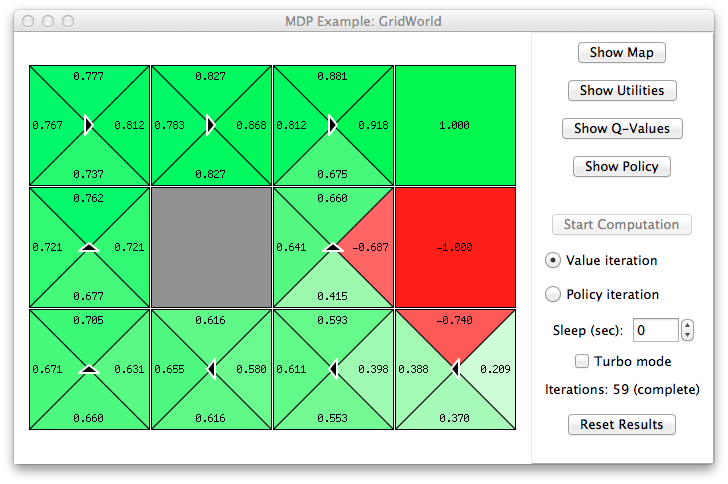
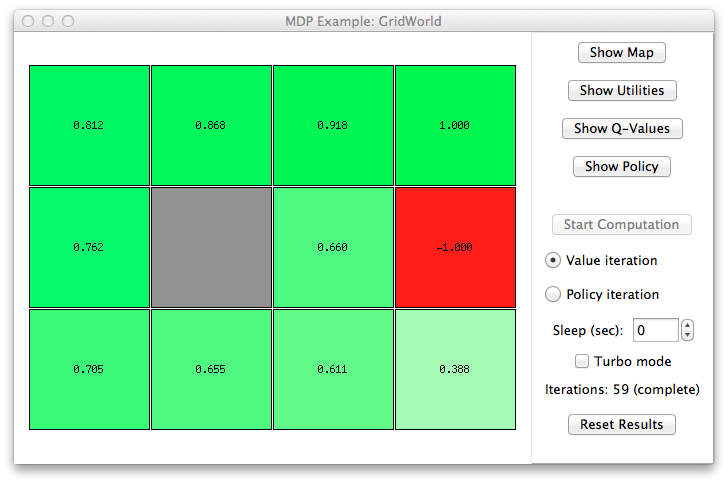
You can try other parameters, to see the possible commands execute the following:
python3.3 main.pyAlso, there is a window that allow you to configure the parameters as you want, you can launch it with the following:
python3.3 main.py gridworldDownload
Try to run the examples and see the code to better understand. In the code you can see other concepts and a lot of code to draw the data, to make the GUI and to debug the Policy Iteration and the Value Iteration.
