With the success of Ruzzle Solver, a lot of users have asked me to publish more informations about it. In this post, I will talk about some methods to realise this type of algorithms. Surely, in the future, I will talk more about its implementation.
We know that in a dictionary there are a fixed number words (for example, in the Italian one, there are 600.000 words). Then, we also know that Ruzzle has a fixed matrix of 4x4 cells. Surely, we are talking about an O(1) algorithm, but not all the ways to solve this problem are the same, the theory and the practice aren’t always the same thing.
Full Enumeration
Assume that we load the set of words into an hashmap. We know that this type of structure has a lookup that, in the average case, requires a time of O(1). However, we have a static dictionary, we don’t need to change it once loaded. We can assume that our hashmap is an array that contains all the words, and that the hash function is perfect (i.e. injective); in this way we can have always a time complexity of O(1). The latter data structure is known in literature with the name: Direct Access Table.
The first algorithm that we can think can search all combination in the matrix, and, for each of them, we can look if it is in the dictionary or not.
We want to estimate the number of lookups at the hashmap. We assume that we have a matrix with distinct letters: we don’t count the words that can be drawn in different ways (this is not much important for now).
The algorithm starts choosing a cell, one of the 16 in the matrix. This cell is the first letter of the word that we are drawing. Now, the algorithm needs to choose one of the adjacent cells to continue. Each central cell has 8 neighbours, the cells in the corners have 3 neighbours, and the ones in the edges have 5 of them. The average is (84+58+34)/16 = 5,25. The possible words of two letters are 15 * 5,25 = 84. From the second step, each neighbour has one other neighbour that we have visited (and that Ruzzle doesn’t allow to use anymore), leading our average to 4,25. All the possible words of three letters that we can draw are 165,25*4,25 = 357. Obviously, the higher is the number of the steps and the smaller is the average of the number of neighbours (due to the visited ones that decrease). With this process, the number of possible words that have at most seven letters already exceeds one million.
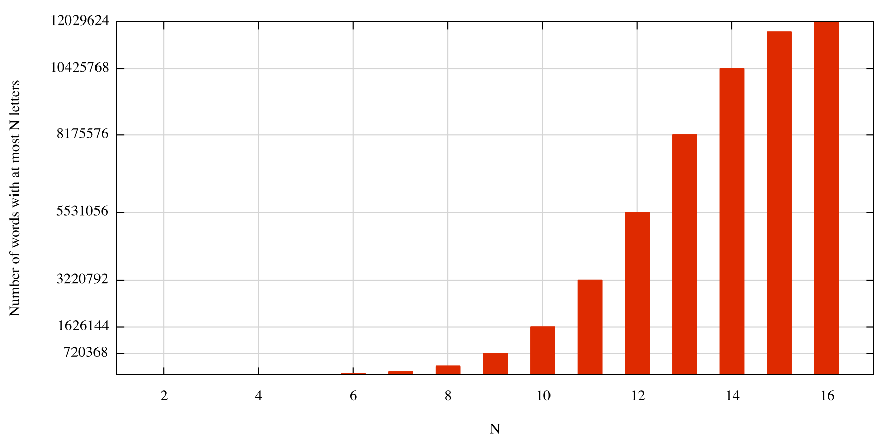
Due to the visited cells, doing an analytical estimation is a little complex. However, with a simple recursive algorithm, we can count the exact number of combinations of the matrix: 12.029.624.

In this picture we can see the trend of possible words in a matrix (assuming a matrix with all distinct letters). Each bar shows the number of possible words that have at most N letters. In other words, it shows the search tree size (up to the level N) of the recursive algorithm that searches all the possible words in the matrix. We can see that the grow seems exponential, but this grow decreases due to the increasing number of visited neighbours.
Hence, this algorithm needs 12 millions of lookups to the dictionary. To put this in real numbers, the simpler algorithm that only counts the number of combinations, without verifying if words are existing or not, takes 2.5 seconds on my laptop.
Active Dictionary
Looking at the higher number of combination that we calculated in the previous algorithm, we can change the role of the dictionary: from passive to active.
Assume that we have our dictionary, and that we read the words one by one. For each of them we only verify if it is in the matrix or not. This method seems reasonable, since the number of existing words is smaller that the number of possible words in the matrix.
This verification is fast. Let’s assume we want to verify if the word “HOME” is in the matrix. First of all, we want search for a cell that contains an “H”. From that cell we want to search for neighbours with a letter “O”. If we found one now we need to verify if there is a neighbour with the letter “M”, and so on. These operations are simple, we only check the letters of the word with the ones in the matrix. We don’t need to have an hashmap, the dictionary is read sequentially.
Again, to put this in numbers, the average time to find all the words that are in the matrix is 150 milliseconds on my laptop. Compared to the previous one, this is already a big step forward.
Branch and Bound
Looking at the first algorithm we can observe something. The lookup for a word “clev” fails, but we must continue the research from this word and up to 15 letters in order to find existing words. For example “clever” is in the dictionary.
To speed up the research, it would be useful to know instead, from the first letters, that the word is not a prefix of any word in the dictionary
. For example, with “xhct” we don’t need to continue to search, we will not find any longer word with that prefix.
Hence, to do this, we need a clever “hashmap”, where we can do prefixes lookups. This type of data structures exists and is widely used, for example in information retrieval. Examples of these are:
Trie
, and
Radix Tree
We expect such an algorithm to be very fast, because the enumeration of all possible combination is rigorously guided, excluding all wrong path, and using very fast lookup. To test this algorithm, I implemented an optimised version of Trie, which is expensive in terms of memory.
To compare this with the other two algorithms in term of time, this algorithm needs, in the average case, less than 1ms to calculate all words in the matrix in my laptop.
Conclusion
We have seen three ways to solve this problem, each of them has pros and cons:
| Algorithm | Time | Time (total) | Memory |
|---|---|---|---|
| Full Enumeration | 2,5sec+ | 2,5sec+ | ~6MB |
| Active Dictionary | 150ms | 170ms | ~0MB |
| Branch and Bound | 1ms | 300ms | ~140MB |
The second method, despite the time of 150ms, is a practical algorithm, where you don’t need to much memory to memorise the dictionary.
The third method is surely faster, but it is expensive in terms of memory, and the algorithm also needs a slow phase where the data structure is getting ready.
